Rethinking Normalization in RNA-seq and ChIP-seq

Get the basics sorted out.

Foreword

I recently work on a project where the data is primarily from an enrichment-based assay. And this is the first time I work with such type of NGS data. Naturally, normalization is the first step after I get a count matrix, and naturally, I would try a library-size-based normalization, i.e. dividing the count of each feature by the total library size (and there could be more sophisticated operations like multiplying by a scalar to make the number looks larger, or accounting for gene length etc, but let’s just call this a library-size-based normalization). But as I think deeper on this general approach, I developed more doubts on it. Is it fair to do so? What if there is some global change between samples? For example in a ChIP-seq experiment, probably in an unlikely scenario, the transcription factor we are looking at binds 2 times more in one sample compared to another sample, after immunoprecipatation, we would get a lot more fragments in that super active sample, how do we justify the idea of libray-size based normaliztion, and how do we check for such a “global” activation? Remember, in reality, as a computational scientist, we only see the numbers in the count matrix, or bam reads, and we don’t have (or shouldn’t have (think double-blined clinical trials)) the knowledge about the ground truth.

Typical RNA-seq experiments

It is always easier to learn from something simpler, and generalize the learning to a more complicated experiment design. In a typcial RNA-seq experiments, we are comparing gene expression beteen sample groups, for example, tumor vs normal, treatment vs control. The differences we observe in library sizes could be resulted from differences in the following¹:

• 1 Loadings of RNA
• 2 Nature of RNA sampels (e.g. you got degraded RNA in a sample)
• 3 Library preparation efficiency (adapther ligation, PCR amplification, etc)
• 4 Sequencing variablity (sequencing efficiency)
• 5 Alignment (low quality reads are filtered)
• 6 Human handling errors that are completely random and untrackable.

Let’s tackle them one by one:

• 1 Loadings of RNA
  • Typically in the context of differential expression analysis, people would start with the same loadings for all the samples, but even without², we can assume proportionality³ and size up or down the samples to the same library size, so basically we do a library size normalization and compare the per-unit (per million) size counts. Most importantly, this won’t be of biological relevance (i.e. we hope different samples to have the same loadings).
• 2 Nature of RNA samples (e.g. comparison groups)
  • Given same loadings (before or after adjustment), it shouldn’t affect the grand total library size. As for compositional biases, we use methods like TMM to take care.
• 3 Library preparation efficiency (adapther ligation, PCR amplification, etc)
  • These biases are considered random. We know their existence, but we can’t tell exactly how much they affect without having spike-in samples.
• 4 Sequencing variablity
  • Same. These biases are considered random. We know their existence, but we can’t tell exactly how much they affect without having spike-in samples.
• 5 Alignment (low quality reads are filtered)
  • Some samples may have more low quality reads than others, and this goes back to our pointer 2.
• 6 Human handling errors that are completely random and untrackable.
  • Same as before, this is not of interest and except for library size normalization, we don’t do anything to address it.

Basically all these biases could potentially change the library size, and usually the experiment is affected by multiple factors. Library-size-based normalization makes us comparing groups in a per unit library size (usually per million) basis, addressing all these biases. Anything that is not random here (except for comparison groups), can be accounted for by batch correction.

Long story short, why is it okay to compare in unit library size? Because the factors that result in library size differences are not of our interest.

Enrichment-based assays

Let’s take a look at a general ChIP-seq experiment workflow:

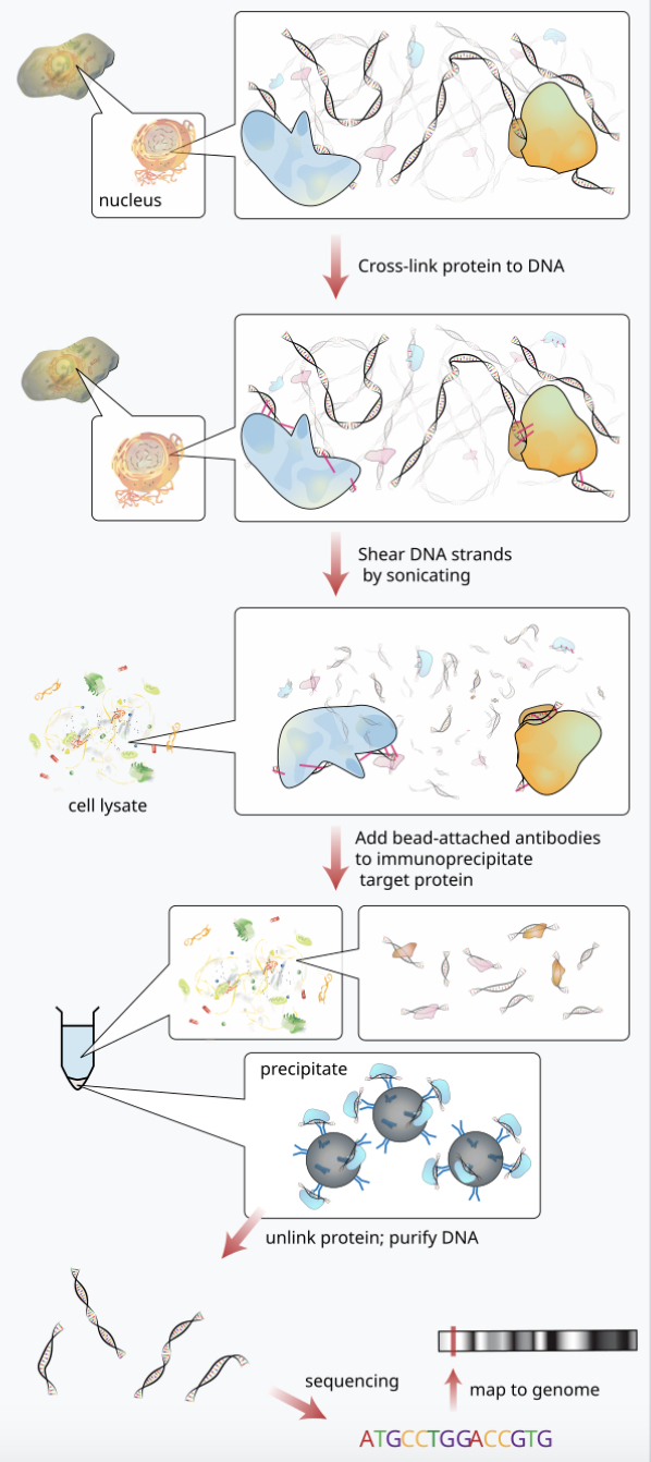
In the immunoprecipitation (IP) step, DNA that were bound by the target protein (e.g. transcription factor) are grabbed (others are washed out) and subjected to sequencing. Imaging we are comparing group A and B, and we start off with the same amount of cells, we cross link, shear DNA strands, we precipitate and unlink DNA from protein, we reach the sequencing step, we would most likely end up with different amounts of DNA material, when libraries are constructed, similar amount of DNA would be loaded to the sequencer such that we lose the informatoin that how much binding happend in total. We can not say enrichment of binding in this site is more in A than B, but we can say enrichment of binding in this site is more in A comparing to A’s other binding sites than in B comparing to B’s other binding sites.

Because of the addtional IP step in ChIP-seq, there are some other sources biases.

• 7 Crosslinking efficiency
• 8 Shearing efficiency
• 9 IP efficiency
• 10 DNA recovery efficiency after IP
• and more

Two major differences from RNA-seq data:

• We often supplement our ChIP samples with an “input sample” as background control.
  • Input samples are processedd in parallel with the ChIP samples but does not undergo immunoprecipitation. Instead, the crosslinked chromatin is reverse-crosslinked, and the DNA is purified directly and sequenced. So it is supposed to be the same as its pairing ChIP sample in all the aspects but for the signals from DNA that are bound to the target proteins.
  • Imaging a chromatin region with no enrichment of binding with the target protein, but it is more open (accessible) compared to other regions. It would be more easily fragmented in the shearing step, and more likely to be bound by proteins non-specifically, including the antibody used in ChIP, also it would be amplified in the sequencing library too. Such regions in the input sample would have higher coverage because they are more accessible. Therefore, input control sample helps us to identify genuine binding sites.
• Peaks are the features in ChIP-seq experiments.
  • In RNA-seq experiments, genes are often the features. In ChIP-seq, we introduce the concept of peaks, which are the regions of signficant enrichment of read counts. Popular tools like MACS2 model the read counts with a poisson distribution and only significantly different from the background (input sample’s distribution if there is the input sample) are considered a peak.
  • After peak calling, you would get a matrix with the rows being peaks, and columns being the samples. The values are read counts mapped to the peaks. You could imagine these reads would be a subset of the total reads. Usually the fraction of Read in Peaks (RiP) is no higher than 20% in transcription factor binding scenario and no more than 60% in histone modifications (need to find reference for this). The reads that are not mapped to any peaks are considered noise that is reflective of the ChIP efficiency.

Knowing the two details of the data, it makes more sense to normalize against the total reads in peaks than the full library size to also account for the ChIP efficiency bias. As I have already said, at this stage we already gave up studying the global absolute shift of signals, we are doing this in relative terms.

Please take a look at the DiffBind tutorial⁴ to see even more details in normalization. They compared full library size with read in peaks, and mentioned background normalization, where larger bins are formed. Coupled with TMM, it can yield more robust results.

Then how do we know if there is a global binding shift?

Experimentally The best practice to have “spike-in” samples (Orlando, David A., et al. “Quantitative ChIP-Seq normalization reveals global modulation of the epigenome.” Cell reports 9.3 (2014): 1163-1170.), which are made of known quantity of exogenous (mostly drosophila when study human samples) DNA or chromatin. They are added to all the samples in the study right before all the processing steps. Unlike the input controls we talked about, they are also immunoprecipitated. Because we know their quantities (amount of bindings) are equal across all the samples, after all the procedures, they should, in theory, yield the same amount of DNA fragments in the final library. Any difference are for sure technical biases, such as variations in immunoprecipitation efficiency, sequencing depth, or library preparation. And these biases are the same biases the actual samples are suffering from. So if we normalize our human samples with the spike-ins we correct for technical biases and isolate true biological signals.

Computationally In the scenario where no spike-ins are availabily, which is unfortunately mose cases I have seen. Computational methods come to rescue. I found a tool called ChIPseqSpikeInFree (Jin, Hongjian, et al. “ChIPseqSpikeInFree: a ChIP-seq normalization approach to reveal global changes in histone modifications without spike-in.” Bioinformatics 36.4 (2020): 1270-1272.) that could be used to study the global shift question. It was tested to be successful for histon modifications but no systematic benchmark was done for other types of ChIPseq experiments.

P.S.

Normalization is a critical yet often overlooked aspect of data analysis. While it may not seem as exciting as employing cutting-edge AI tools—especially in today’s research climate—it remains a cornerstone of robust dicovery.

I initially aimed to cover normalization in single-cell RNA-seq and proteomics data analysis as well, including some hands-on examples. However, this blog post has already grown quite lengthy. I’ll save those topics for a future installment, so stay tuned!

1. I’m trying to list all the possible sources in the order of the experiment workflow, and trying to be mutually exclusive. ↩

2. If the loadings are off by too much, you would imagine the variance of gene counts between samples would be quite different, and all the uncontrollable factors would have influenced the samples at different magnitudes. ↩

3. We assume if we use two times the original loading, the reads and counts would be two times the original resutls. This sounds like a strong assumption, but it is also what we assume when we conduct any NGS experiment. It is wild if we repeat the analysis with different loadings and the conclusion changes qualitatively. But it is a good idea to keep the loadings the same between samples, especially when you want to compare them, as footnote 2 points out. ↩

4. I don’t fully agree with their recommendation of using full library size. It seems they are still trying to make an absolute differential binding conclusion knowing the raw data trend is explainable by both biological difference and technical artefacts. ↩